Suitability Modeling

Goal and Objectives

It is important to explore all the different types of geoprocessing tools in ArcGIS in order to build models to solve real life issues.  During this semester, we have been looking at sand mines in western Wisconsin more from the business side and how the companies can become more efficient.  It is also important to build models for how the surroundings of the sand mines are impacted from a suitability, environmental, and cultural standpoint in Trempealeau County.  This lab looks to answer those questions through the following objectives:

1. Generate spatial data layer to meet geologic criteria
2. Generate spatial data layer to meet land use land cover criteria
3. Generate a spatial data layer to meet distance to railroads criteria
4. Generate a spatial data layer to meet the slope criteria
5. Generate a spatial data layer to meet the water-table depth criteria

Methods

Find suitable land for the geologic criteria
The two geologic units that are mined for frac sand are from the Jordan Formation and the Wonowac Formation.  For the first map, those desired areas of geologic formations are made into one color while the rest of the geologic units are made in another color.  This helps show where the mine able areas are.

Find suitable land for the land use criteria
By comparing the National Land Cover Data and the map the was created in the previous step, I noticed that the land cover in the areas common for frac sand mining is deciduous forest.  This type of land is dominated by trees that are generally greater than 5 meters tall, and greater than 20% of total vegetation cover.  More than 75% of the tree species shed foliage simultaneously in response to seasonal change.

Find suitable land for the proximity to railroads criteria
To see the distance away from each railroad terminal in every direction, the Euclidean distance tool can be used.  The result shows a nice radial map that gives a quick visual representation of distances to each railroad terminal.

Find suitable land for the slope criteria
It is important to find the slope in an area especially for a business like a sand mine.  The 3-D analyst tool "Slope" was used to find this factor.  A percent rise was used for the output measurement.

Find water table depth
The attribute that shows water depth in the coverage file is "wt_elev" which is the water table elevation.  The tool used to show the water table depth properly is the "Topo to Raster" tool.  The coverage file for the water table is originally imported into ArcGIS as a vector feature class.  This tool allows us to see continuous data for water table depth, which is probably more realistic than just a polyline.

Results

Find suitable land for the geologic criteria

The purple areas show where the Jordan and the Wonowac Formations are in western Wisconsin, which have proven to be the best units to find frac sand in.  All other geologic formation are shown in blue.

Find suitable land for the land use criteria

Based on National Land Cover Data, the yellow areas show land that possibly has go land cover for frac sand.  I have reclassed all other types of land cover in red.

Find suitable land for the proximity to railroads criteria

Red dots represent the railroad terminals and the colors represent the distance from each railroad termainal.

Find suitable land for the slope criteria

Slope that was calculated from elevation data.  The lighter colors represent lower elevations.  The numbers rank the elevation values; the higher the elevation, the higher the rank.

Find water table depth

This is a map of Trempealeau County that shows the depth of the water table.

Sources

·         http://www.mrlc.gov/nlcd01_leg.php

 http://wisconsingeologicalsurvey.org/gis.htm

Network Analysis

Goals and Objectives

Network Analysis is a very useful tool that shoots to help transportation challenges.  With this tool, one can perform a point to point routing, calculate driving times, show traffic maps, etc.  With this lab, we wanted to calculate a route for sand mining trucks to take the frac sand from the mine to a railroad, seeing as the railroad is the most efficient way to transport the sand to desired areas.  To do this, it was essential to find the closest railroad stop to each sand mine.  For these large trucks to transport this sand, it costs a lot of money, not only in gas prices, but also in wear and tear on the roads.  This is another important reason to find the shortest driving distance necessary to transport the sand.  Another goal is to keep track of the work flow using a data flow model throughout the lab.

Methods

In ArcGIS, ModelBuilder was utilized to run the closest facility tool for this network analysis.

Data flow model for running network analysis with the closest facilities tool.

First the streets were made the input on a "Make Closest Facility" tool with the "travel to" option.  This is because we want to travel by roads to the closest railroad terminal.  The next tool was "Add Location"  which is where we added the sand mines that were not close to railroad terminals.  Using the "Solve" tool at this point gives the railroad terminal that is closest to each sand mine that is not already on a railroad terminal.  The "Select Data" tool that comes next allows you to input that closest facilities layer and then calculate a route for how to get from each sand mine to a railroad terminal.  The "Copy Feature" allows you to make this route its own feature class.  From there you can view specific information about each route that a truck would take from each sand mine to the nearest railroad terminal.

This is part of the table that is created when making the route output as its own feature class.

Efficiency is everything with a business like this, and costs are very important.  The roads that these large trucks need to travel on to get to the railroad terminals start to wear down after awhile.  A cost of 2.2 cents per miles accounts for this wear.  Other costs to think about are gas prices.  According to http://www.gasbuddy.com/Gas_Prices/Wisconsin/index.aspx, the highest gas price in this general area is around $3.15 per gallon.  The website http://www.ehow.com/facts_5844120_fuel-mileage-information-semi-trucks.html says that the new designs of semi trucks get about 7 miles per gallon.

Results 

Map showing the fastest route from sand mines to a railroad terminal.

The total distance traveled by a single sand truck from each sand mine to the nearest railroad terminal was found to be 778.883 km.  The total amount spent in gas was $27,639.40 and the total amount accounted for the wear and tear on the road was calculated to be $1,064.75.  Adding these values together gives a grand total of $28,704.15 spent on getting one truck load of sand from each mine to its nearest railroad terminal.

Spreadsheet of costs for hauling the mined sand from the sand mines to the closest railroad terminal.

Conclusions

Network analysis can be a very important tool for any company that needs to deliver a product to its customers.  With just a few quick tools, I have shown the most efficient way for the sand mines in western Wisconsin to get their product from the mine to the closest railroad terminal, where it can then be transferred more directly and efficiently to the customer.  Not only can time be saved, but money too, as demonstrated in the last step of this lab.

Resources

http://www.gasbuddy.com/Gas_Prices/Wisconsin/index.aspx

http://www.ehow.com/facts_5844120_fuel-mileage-information-semi-trucks.html

Acquiring Data - An Essential First Step

Goals and Objectives

An important part of any project is obtaining the data.  If one is not getting data from credible places, any analysis may not be justified or worthwhile.  The main goal of this lab exercise was to become familiar with the process of downloading data from different sources on the internet, importing data to ArcGIS, joining data together, and projecting data from these different sources into a single coordinate system that makes sense while building and designing a geodatabase to store the data.

General Methods

The first site that data were acquired was the nationalatlas.gov, which is where the DEM data was downloaded.  DEM (digital elevation model) data can easily show high and low areas in the area of interest.  By default, the areas of high elevation are white and low elevations are shown in black.

Two DEM files that were mosaicked together to form a seamless image. 

One important site used to obtain data was the USGS National Map Viewer.  

This is the first view of the National Map Viewer from the United States Geological Survey page.

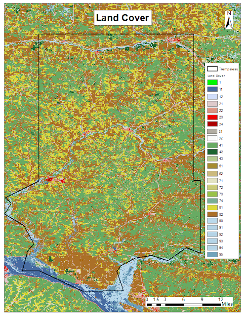
This is a very useful site for many different applications of data, such as man made structures (like public attractions, medical facilities, education, etc.), transportation information, governmental boundaries, hydrography data, land cover, elevation, and imagery.  We used land cover data in the Trempeleau County area.

This is a map showing the land cover data from the USGS.  Not all of the categories are broken down in the legend on the side, only the categories that had a distinct difference from one another in their color.

We also used the USDA NRCS Web Soil Survey to download SSURGO data, which just stands for soil survey geographical.

This is what the general soils map of Tremeleau County looks like.  I did not include a legend because the breakdown of the soils is too complex in this system.

This a more zoomed in view of an area in Trempeleau County (reference map) just to show how detailed the soil can be over a small area and how complex the patterns can be.

Results

In order for all the data to show up in its proper location, each piece of data needed to be in the same coordinate system.  To do this, the tool define projection must be run on all the data using the same coordinate system.  I decided to use the NAD_1983_HARN_WISCRS_Trempealeau_County_Meters because it is focused around the study area of Trempeleau County.  Once all the data have a defined projection, then the project tool must be run on all the data, so they all show up in the data frame in the same coordinate system, and so that everything appears to be in the correct location relative to each other.

Here are both maps of the land cover data and the soil survey data overlain by the main roads layer in bright red.

Conclusion

This lab opened up the door for endless future possibilities at retrieving data.  There are so many resources to be tapped, and that number is increasing as technology becomes more and more available to the average person.  While putting this data together, I also worked on building a geodatabase with many different file types.  A lot of files can be created once data needs to have a defined projection and needs to be projected, so it is important to keep organized for these projects.  Getting data from multiple sources means the data will probably not be in the same projection, so it is essential to pay attention to details like that when showing many kinds of data.

Geocoding Sand Mines for Hydraulic Fracturing in Western Wisconsin

Goal

In this lab, we were to acquire raw data of current or prospective sand mines in Western Wisconsin, find the location of each mine given the incomplete data, compare your location to locations other students chose, and examine the error.

Methods

In order for the mines to be geocoded in ArcGIS, they would each need to have a complete address, which was not the case for every mine site.  If addresses were not provided, I used imagery from Google Earth and other internet searches to try to find the exact address of each sand mine that is active, in process, or proposed.  The main components of the location that are needed are the facility address, community (city), zip code, and the state.  If this information is not provided, and it cannot be found any other way, a tool can be used in ArcGIS that allows you to pick an address from the map, where you can click your mouse on a map, and it will give an address for you, which is found in the geocoding toolbar.

Figure 1:  Table of the mines I was assigned after the addresses were found.

Once all the information is filled in for each mine, you can match the information to real space in the program.  A window something like the one below will show how closely matched your data is.

Figure 2:  A simplified example of the geocoding table used to match proximity of your data to real space.  

Once there is a 100% match, the geocoding process should be successful.  After this point, each student made a shapefile of all their mines (each student had about 14 mines), making sure that their unique field ID has been preserved through their geocoding process.  From here, all the shapefiles were merged together, not including the shapefile of the mines that I geocoded.  A query can be done to select only the mines that matched the unique field ID of the mines I was assigned.  Once those selected mines are made into their own feature class, the point distance tool can be run the see how close my location for each mine was compared to locations other students chose for the same mine.

Results

Figure 3:  A small scale map of my mine locations compared to other student locations of the same mine.

The point distance tool creates a table that calculates the distance between one of my mines, which is shown as a single point, and the nearest mine that was located by another student.  Each mine is given an input_FID in the table that shows the distances from my mine to everyone else's mine with the same ID.  The highlighted area in the table below represents the distance from my mine location to other students' mine locations.  The last column shows this distance in kilometers.

Figure 3:  This is part of the table that is created from the point distance tool.  The highlighted area shows the distance of my location for that mine compared to where my peers put the same mine.

When looking through the data, I looked within each input_FID for the shortest distance calculated and compiled those in a separate table to see the variety in distances between my mine locations and my peers' mine locations.

Figure 4:  This table shows a summary of the shortest distance between my mine locations and the location that a peer chose for the same mine.

The shortest distance found between two points of the same mine was about 9 kilometers, and the greatest distance between two points of the same mine was about 75 kilometers.

Conclusions

I think the largest source of error here deals with inherent errors of how people geocoded their mines.  They maybe found an address that was incorrect or for a different mine.  If they had to pick an address from the map, it is possible that they were zoomed in to the wrong area, or found the wrong location for that particular mine.  Since there are so many sand mines that are being implemented in Western Wisconsin, it could be easy enough to choose the wrong one if you do not have exact address information (data automation and compilation, Table 4.1, Lo, Chapter 4).  The only operational error I could see happening would be with the point distance tool.  The program only calculates a distance between two points that are closest to each other.  The user does not have any way of knowing which two points it used for this calculation.  In this case, the tool could have calculate a distance between two different mines.  In order to figure this out, you could do a quick draw between the two points that you want to know the difference between, and see if the calculation was close or not.

Citations
Lo (2001).  Data Quality and Data Standards, Ch. 4, 105-108.

Sand Mining in Western Wisconsin - Why do we care?

Since the beginning of time, the human race has been taking what they need from the Earth in order to survive.  Over time these needs have gotten more extensive.  We now need to look for different options to provide for our greedy habits.  The means to energy has gotten more slim with the development of motorized vehicles and other technologies.  The relatively recent idea of hydraulic fracturing has been explored to provide a source of natural gas.

The process of hydraulic fracturing provides an innovative way to extract natural gas out of the ground.  Shale is a type of rock that commonly holds natural gas.  It forms in relatively thin sheet like layers but is good for containing natural gas due to its impermeability.  This means fluids cannot pass through this layer in the ground.  A small amount of explosives are used to crack open the shale rock.  Sand is then placed into those cracks to keep the rock open long enough to extract the gas within it.  

A process like this may seam rather simple, but a certain type of sand must be used in order for this to work properly.  The sand grains must be about the same size, otherwise the opening in the rock will not be the same throughout the fracture.  The sand grains must also be well rounded.  If angular grains are sent into a fracture,  the grains may be wedged in the opening at an obscure angle, which would also cause the opening to be irregular.  Each sand grain must also have a relatively high strength to them.  The shale rock that the sand is being sent to is relatively deep in the ground and feels a lot of pressure from the overlying rock.  This high pressure could cause the opening to collapse if the sand grains are not strong enough to hold it open.  On Moh's hardness scale, the mineral quartz is about a 7 (the highest value is 10).  This mineral provides the strength needed to keep a fractured shale open.  The Cambrian and Ordovician aged sand, most commonly from the Jordan Sandstone and the Mt. Simon Formation, found in western Wisconsin fulfills these criteria pretty well.

Even though hydraulic fracturing appears to be a solution towards our high need for energy, there are environmental impacts to consider.  Any type of mining takes a toll on the air quality in surrounding areas.  The chemicals used at a mine site may become airborne and blow to surrounding residential areas.  The dust from blasting at a site may also get carried to residential areas.  A fluid is used to help get the sand grains wedged into the cracks of the shale rock.  People worry that this fluid gets into the ground water when sending it down into the ground and bringing it back up to the surface.  Some people believe that this fluid affects their drinking water and that they may be ingesting chemicals from this process.  This fracking fluid may also be harmful to the environment because of the chemicals that it contains.  It is possible to have this fluid enter surface water in streams, rivers, or lakes.  Heavy research is done to look for biodegradable chemicals to use.  Great caution and intense reclamation is done as well to ensure safety for the environment.

Another issue is the affect that transportation of the sand has on the environment.  Large trucks are needed to transport the sand from the mining site to the railroad where the sand is further transported.  The roads that the trucks travel need to be replaced more often than normal roads due to the heavy loads that are transported along that route.  This can get expensive for the state if many roads need replacing often.

GIS can be used to help solve some of these issues.  Through this program, we can explore the areas subjected to environmental impacts, monitor how water flows in and around the mining site, and look at how the roads are affected by transportation.

I am a geology major at the University of Wisconsin-Eau Claire.  Kent Syverson is the leading professor in the geology department who studies hydraulic fracturing and sand mining.  My knowledge of the material comes from his various teachings.